
Introduction
In the previous post, we focused on transforming raw Windows authentication logs into a compact set of behavioral features. That step was intentionally heavy on data engineering, because anomaly detection only works if the underlying data has structure.
At this stage, we are no longer dealing with logs.
We have:
- a numerical feature space,
- one row per authentication event,
- and signals that describe how users authenticate rather than what they authenticate to.
This post covers the second stage of the pipeline: learning what normal authentication behavior looks like using an unsupervised machine learning model.
Two clarifications upfront:
- This post is not about alerts or SOC workflows.
- This post is not about detecting attacks directly.
The goal is simpler:
How unusual is this authentication event compared to normal behavior?
Everything else is built on top of that signal.
Problem Framing: Behavioral Anomaly Detection Without Labels
Authentication anomaly detection is a label-poor problem.
In real environments:
- reliable labels for malicious logins rarely exist,
- many suspicious-looking events are benign,
- and many attacks deliberately blend into normal behavior.
Because of this, supervised approaches are usually impractical.
Instead of classifying events as good or bad, we reframe the problem:
Learn what normal authentication behavior looks like, and measure deviations from that baseline.
This framing drives all design decisions that follow.
What This Model Does (and What It Does Not)
A common mistake in security ML is equating anomalies with attacks.
They are not the same.
Examples of normal but unusual behavior include:
- users repeatedly mistyping passwords,
- administrators logging in from many IPs,
- legitimate VPN reconnections.
Conversely, many real attacks appear statistically normal.
For this reason, the model in this post:
- does not classify attacks,
- does not enforce policy,
- and does not replace rule-based detections.
What it provides is a continuous anomaly score that reflects behavioral deviation.
Authentication failures illustrate this well.
Failures are often part of normal behavior:
- some users fail consistently,
- some systems retry authentication by design.
Excluding failures from training would artificially narrow the learned behavior space and increase false positives. Instead, failures are treated as contextual signals, not anomalies by default.
Scope and Intent
This work intentionally focuses on authentication events only.
Authentication telemetry provides:
- strong behavioral regularities,
- wide availability across environments,
- and a clean starting point for anomaly detection.
This scope is a proof of concept, not a limitation.
The same pipeline can be extended to include:
- process creation,
- service activity,
- PowerShell execution,
- or lateral movement indicators.
As additional signals are added, the notion of “normal behavior” becomes richer, while the modeling approach remains the same.
Input Data and Feature Space
Before introducing a model, it is important to clarify what the model actually sees.
The autoencoder does not operate on raw logs, usernames, or IP addresses. It operates on a numerical feature space derived from authentication behavior.
Each authentication event is represented by:
hourdayofweekis_failureuser_login_countuser_ip_count
This feature set is intentionally compact. The goal is to encode behavioral regularities, not full event semantics.
Why Identifiers Are Excluded
A common question is:
Why not include usernames or IP addresses directly?
Because identifiers do not generalize.
They are:
- high-cardinality,
- environment-specific,
- and meaningless outside local context.
Including them would encourage memorization rather than learning behavior.
Instead, identifiers are used indirectly to derive signals such as activity frequency and IP stability. Raw identifiers remain available outside the model for investigation and explainability.
From Events to Behavior
Raw event fields answer what happened. Behavioral features answer how this event relates to past behavior.
A failed login, an off-hours login, or a new IP address is not inherently suspicious. What matters is how these properties combine over time and frequency.
This shift — from events to behavior — makes unsupervised detection feasible.
Preparing the Feature Space for Modeling
Although all features are numerical, they behave very differently.
Temporal features are bounded. Frequency-based features exhibit heavy-tailed distributions, which is typical in authentication telemetry.
If left untreated, these differences would cause reconstruction loss to be dominated by a small subset of features.
To address this:
- frequency-based features are stabilized using a
log1ptransform, - features are then normalized using standard scaling.
This does not remove rare events; it mainly reduces scale effects so that one count-based feature cannot dominate the reconstruction loss.
Authentication failures are intentionally retained, as they are part of normal behavior.
At the end of this step, the feature space is numerically stable and suitable for reconstruction-based learning.
Why an Autoencoder?
The problem is now well defined:
- unlabeled data,
- dominant normal behavior,
- rare and diverse deviations.
Autoencoders fit this setting naturally.
They learn to reconstruct typical behavior and produce a continuous reconstruction error when behavior deviates from what was learned.
They:
- require no labels,
- adapt to behavioral patterns,
- and remain simple enough to reason about.
The autoencoder used here is intentionally minimal and serves as a baseline for later comparison with other unsupervised techniques.
With the modeling choice justified, we can now move from concepts to implementation.
The next section walks through the training notebook step by step.
Training an Autoencoder for Authentication Behavior
All experiments in this post were conducted using a notebook.
Rather than presenting the notebook verbatim, this section follows its structure step by step and explains the rationale behind each stage.
The objective is not to tune a model aggressively, but to demonstrate a clean, reproducible baseline for unsupervised behavioral detection.
Step 1 — Loading and Validating the Feature Dataset
The first step of the notebook focuses on validating the feature dataset produced in Part 1.
At this stage, no modeling decisions are made.
The objective is to ensure that the data is structurally sound, internally consistent, and safe to use as input for an unsupervised model.
Loading the Feature Matrix
The feature dataset is loaded from a Parquet file generated during the feature extraction phase:
FEATURE_PATH = "../data/auth_features.parquet"
X = pd.read_parquet(FEATURE_PATH)

X.head()
Each row corresponds to a single authentication event, and each column represents a behavioral feature derived from Windows authentication logs.
Dataset Shape and Data Types
Before proceeding, the overall shape and data types are inspected:
print("Shape:", X.shape)
print("Columns:", X.columns.tolist())
print("\nDtypes:\n", X.dtypes)
Shape: (26417, 5)
Columns: ['hour', 'dayofweek', 'is_failure', 'user_ip_count', 'user_login_count']
Dtypes:
hour float64
dayofweek float64
is_failure float64
user_ip_count float64
user_login_count float64
dtype: objectThis confirms:
- the number of events available for training,
- the exact set of extracted features,
- and that all features are numerical.
Ensuring consistent data types at this stage avoids subtle issues later during scaling or model training.
Explicit Feature Selection
To guarantee consistency with the feature engineering performed in Part 1, the expected feature set is defined explicitly:
FEATURE_COLUMNS = [
    "hour",
    "dayofweek",
    "is_failure",
    "user_ip_count",
    "user_login_count",
]
The dataset is then validated against this expected schema:
missing = [c for c in FEATURE_COLUMNS if c not in X.columns]
extra = [c for c in X.columns if c not in FEATURE_COLUMNS]

if missing:
    raise ValueError(f"Missing columns in parquet: {missing}")
if extra:
    print(f"Warning: extra columns found (ignored): {extra}")
This defensive check ensures that:
- no required features are missing,
- no unexpected columns are silently introduced.
The feature matrix is then reordered explicitly:
X = X[FEATURE_COLUMNS].copy()This guarantees a stable and reproducible feature order across experiments.
Missing and Infinite Values
Before any modeling step, the dataset is checked for invalid values:
na_counts = X.isna().sum()
print("Null counts:\n", na_counts)

is_inf = np.isinf(X.to_numpy()).sum()
print("\nNumber of +/-inf values:", is_inf)

if na_counts.any() or is_inf > 0:
    raise ValueError("Found NaNs or infinite values. Fix before modeling.")
These checks catch common data issues early, such as:
- missing values introduced during feature extraction,
- invalid values caused by incorrect transformations.
Failing fast at this stage prevents undefined behavior during training.
Range Validation for Bounded Features
Several features are expected to lie within strict bounds:
hour: 0–23dayofweek: 0–6is_failure: binary (0 or 1)
These constraints are validated explicitly:
bad_hour = ~X["hour"].between(0, 23)
bad_dow = ~X["dayofweek"].between(0, 6)
bad_fail = ~X["is_failure"].isin([0, 1])

print("Bad hour rows:", bad_hour.sum())
print("Bad dayofweek rows:", bad_dow.sum())
print("Bad is_failure rows:", bad_fail.sum())

if bad_hour.any() or bad_dow.any() or bad_fail.any():
    display(X[bad_hour | bad_dow | bad_fail].head(20))
    raise ValueError("Range check failed. Fix feature extraction before modeling.")
This step validates that feature extraction logic has preserved semantic correctness.
Descriptive Statistics
A high-level statistical summary is then computed:
X.describe().T| Feature | count | mean | std | min | 25% | 50% | 75% | max |
|---|---|---|---|---|---|---|---|---|
| hour | 26417.0 | 15.558845 | 5.703017 | 0.0 | 13.0 | 17.0 | 19.0 | 23.0 |
| dayofweek | 26417.0 | 1.948859 | 1.454149 | 0.0 | 1.0 | 2.0 | 3.0 | 5.0 |
| is_failure | 26417.0 | 0.000644 | 0.025360 | 0.0 | 0.0 | 0.0 | 0.0 | 1.0 |
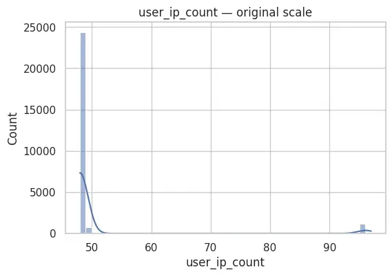
| user_ip_count | 26417.0 | 50.302797 | 10.199039 | 48.0 | 48.0 | 48.0 | 48.0 | 97.0 |
| user_login_count | 26417.0 | 1056.680660 | 0.835593 | 1056.0 | 1056.0 | 1056.0 | 1057.0 | 1059.0 |
This summary shows that temporal features are bounded as expected (hour in [0, 23], dayofweek in [0, 5] in this dataset), while the frequency-based features take a narrow range here (e.g., user_login_count is tightly concentrated around ~1056 and user_ip_count around ~48–97).
Note: this dataset is synthetic, so count-based features are much less variable than what you would typically see in a production environment.
At this point, no transformations are applied. The goal is simply to understand the raw feature behavior.
Feature Correlation
Finally, linear correlations between features are examined:
corr = X.corr()

plt.figure(figsize=(6, 5))
sns.heatmap(
    corr,
    annot=True,
    cmap="coolwarm",
    center=0,
    fmt=".2f"
)
plt.title("Feature correlation matrix (Pearson)")
plt.show()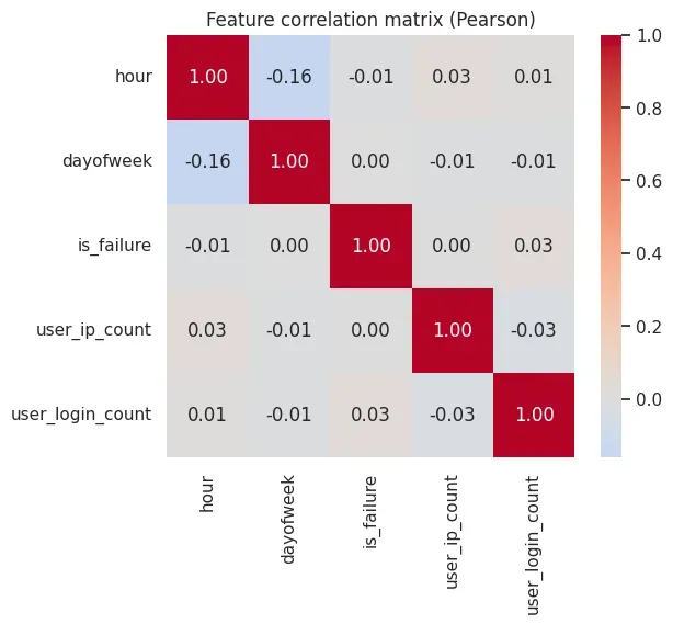
The correlation heatmap suggests that no single feature is perfectly correlated with the others (no values close to ±1), which is a good sign: each feature contributes some independent signal to the model.
Preparing the Dataset for Modeling
After validation, the full dataset is retained for training:
X_all = X.copy()
print("Total events used for training:", len(X_all))
Total events used for training: 26417At this point, the feature space has been validated but not modified.
The next step focuses on conditioning the feature distributions to make them suitable for reconstruction-based learning.
Step 2 — Conditioning, Normalization, and Dataset Splitting
Once the feature space has been validated, the next step is to prepare it for model training.
This stage does not introduce any modeling logic yet.
Its purpose is to ensure that the numerical properties of the data are compatible with neural network training.
Why Conditioning Is Necessary
Although all features are numerical, they do not behave in the same way.
From the previous step, two important observations emerge:
- temporal features (
hour,dayofweek) are bounded and well behaved, - frequency-based features (
user_login_count,user_ip_count) are heavy-tailed and skewed.
If left untreated, these differences would cause the reconstruction loss to be dominated by frequency-based features.
For this reason, frequency stabilization is applied before normalization.
Log-Transforming Frequency-Based Features
The following features represent counts:
user_login_countuser_ip_count
A logarithmic transformation is applied to compress extreme values:
COUNT_COLS = ["user_login_count", "user_ip_count"]

X_tf = X_all.copy()

for c in COUNT_COLS:
    X_tf[c] = np.log1p(X_tf[c])
This transformation:
- preserves ordering,
- reduces skew,
- and prevents extreme values from dominating the loss.
It does not remove rare behavior — it simply expresses it on a more learnable scale.
Verifying the Effect of the Transformation
After transformation, the distributions of the frequency-based features are re-examined:
X_tf[COUNT_COLS].describe().T| Feature | count | mean | std | min | 25% | 50% | 75% | max |
|---|---|---|---|---|---|---|---|---|
| user_login_count | 26417.0 | 6.963833 | 0.000790 | 6.96319 | 6.96319 | 6.96319 | 6.964136 | 6.966024 |
| user_ip_count | 26417.0 | 3.924745 | 0.145015 | 3.89182 | 3.89182 | 3.89182 | 3.891820 | 4.584967 |
The resulting statistics confirm that:
- ranges are compressed,
- extreme values are reduced,
- and the feature space is numerically more balanced.
At this stage, no other features are modified.
Train / Validation Split
Although the task is unsupervised, a validation set is still required.
The validation split is used to:
- monitor convergence,
- detect overfitting,
- and enable early stopping.
Both splits represent the same underlying behavior distribution.
from sklearn.model_selection import train_test_split

X_train, X_val = train_test_split(
    X_tf,
    test_size=0.2,
    random_state=42,
    shuffle=True,
)

print("Train shape:", X_train.shape)
print("Validation shape:", X_val.shape)
Train shape: (21133, 5)
Validation shape: (5284, 5)No filtering is applied at this stage:
- authentication failures are included,
- rare behavior is preserved,
- and the model is exposed to the full range of normal behavior.
Feature Normalization
Neural networks are sensitive to feature scale.
After conditioning, features are normalized using standard scaling:
from sklearn.preprocessing import StandardScaler

scaler = StandardScaler()

X_train_scaled = scaler.fit_transform(X_train)
X_val_scaled = scaler.transform(X_val)
X_all_scaled = scaler.transform(X_tf)
The scaler is fitted only on the training set, then applied consistently to validation and inference data.
This avoids data leakage and ensures that the learned notion of “normal” reflects what the model actually saw during training.
Sanity Check After Scaling
As a final validation step, the scaled training data is inspected:
pd.DataFrame(
    X_train_scaled,
    columns=X_train.columns
).describe().loc[["mean", "std"]]| Statistic | hour | dayofweek | is_failure | user_ip_count | user_login_count |
|---|---|---|---|---|---|
| mean | -1.075918e-16 | 2.790661e-17 | 5.715812e-18 | 3.802024e-15 | 8.857132e-13 |
| std | 1.000024e+00 | 1.000024e+00 | 1.000024e+00 | 1.000024e+00 | 1.000024e+00 |
The scaled training set has mean ~0 and std ~1 for every feature (small e-16 values are normal floating-point noise), confirming that scaling was applied correctly.
Outcome of This Step
At the end of this phase:
- all features are numerically stable,
- scale differences have been removed,
- skewed distributions have been compressed,
- and the dataset is ready for PyTorch.
The next step introduces the autoencoder architecture and training procedure.
Step 3 — Training a Simple Autoencoder in PyTorch
With the feature space conditioned, normalized, and split into train/validation sets, we can train an autoencoder.
The purpose of this model is not classification.
It learns to reconstruct typical authentication behavior and will later be used to compute a reconstruction error score.
PyTorch Setup (Device and DataLoaders)
First, we import PyTorch components and select a device (GPU if available, otherwise CPU):
import torch
from torch import nn
from torch.utils.data import DataLoader, TensorDataset

device = torch.device("cuda" if torch.cuda.is_available() else "cpu")
device
Next, we wrap the scaled NumPy arrays into PyTorch datasets and dataloaders.
Dataloaders allow training in mini-batches, which:
- improves training stability,
- reduces memory usage,
- and speeds up optimization.
train_ds = TensorDataset(torch.tensor(X_train_scaled, dtype=torch.float32))
val_ds   = TensorDataset(torch.tensor(X_val_scaled, dtype=torch.float32))

train_loader = DataLoader(train_ds, batch_size=256, shuffle=True)
val_loader   = DataLoader(val_ds, batch_size=256, shuffle=False)
Autoencoder Architecture
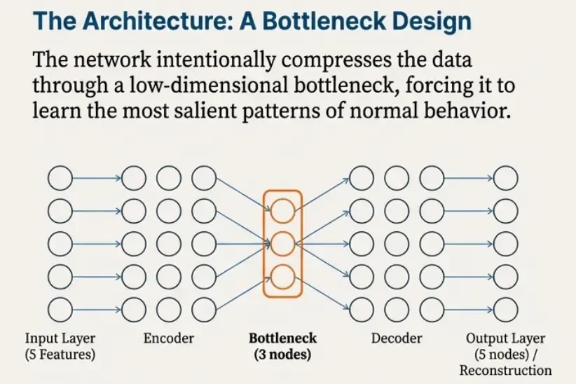
The input space is only 5-dimensional. A deep or complex network would be unnecessary and harder to reason about.
We use a small architecture that is intentionally easy to explain:
- Encoder: 5 → 16 → 3
- Decoder: 3 → 16 → 5
The 3-dimensional bottleneck forces the model to learn a compact representation of normal behavior.
class Autoencoder(nn.Module):
    def __init__(self, input_dim=5, hidden_dim=16, latent_dim=3):
        super().__init__()

        self.encoder = nn.Sequential(
            nn.Linear(input_dim, hidden_dim),
            nn.ReLU(),
            nn.Linear(hidden_dim, latent_dim),
        )

        self.decoder = nn.Sequential(
            nn.Linear(latent_dim, hidden_dim),
            nn.ReLU(),
            nn.Linear(hidden_dim, input_dim),
        )

    def forward(self, x):
        z = self.encoder(x)
        x_hat = self.decoder(z)
        return x_hat
Instantiate the model:
model = Autoencoder(
    input_dim=len(FEATURE_COLUMNS),
    hidden_dim=16,
    latent_dim=3
).to(device)

model
Loss Function and Optimizer
To train an autoencoder, we minimize reconstruction loss.
Mean squared error (MSE) is used because:
- it directly measures reconstruction quality,
- it penalizes large reconstruction mistakes,
- and it produces a continuous error signal suitable for anomaly scoring later.
We optimize using Adam, with a small weight decay term for regularization.
criterion = nn.MSELoss()
optimizer = torch.optim.Adam(model.parameters(), lr=1e-3, weight_decay=1e-5)
Training Loop (Train + Validation)
Training proceeds in epochs.
At each epoch:
- we update model weights using the training set,
- we evaluate reconstruction loss on the validation set.
This provides a sanity check that the model generalizes beyond the training batch distribution.
A helper function runs one epoch in either training or evaluation mode:
def run_epoch(model, loader, train: bool):
    model.train(train)

    total_loss = 0.0
    n = 0

    for (xb,) in loader:
        xb = xb.to(device)

        if train:
            optimizer.zero_grad()

        xb_hat = model(xb)
        loss = criterion(xb_hat, xb)

        if train:
            loss.backward()
            optimizer.step()

        total_loss += loss.item() * xb.size(0)
        n += xb.size(0)

    return total_loss / n
Now we train the model and track train/validation loss:
EPOCHS = 50

train_losses = []
val_losses = []

for epoch in range(1, EPOCHS + 1):
    train_loss = run_epoch(model, train_loader, train=True)
    val_loss   = run_epoch(model, val_loader, train=False)

    train_losses.append(train_loss)
    val_losses.append(val_loss)

    print(f"Epoch {epoch:02d} | train={train_loss:.6f} | val={val_loss:.6f}")
Epoch 01 | train=0.978410 | val=0.716642
Epoch 02 | train=0.750922 | val=0.506557
Epoch 03 | train=0.517377 | val=0.297333
Epoch 04 | train=0.325818 | val=0.161109
Epoch 05 | train=0.228896 | val=0.109804
Epoch 06 | train=0.169867 | val=0.081227
Epoch 07 | train=0.114129 | val=0.058324
Epoch 08 | train=0.065550 | val=0.042978
Epoch 09 | train=0.042997 | val=0.032912
...Training Curve (Convergence Check)
A training curve is plotted to confirm that the model learns stably and does not overfit.
plt.figure(figsize=(6, 4))
sns.lineplot(x=range(1, len(train_losses) + 1), y=train_losses, label="train")
sns.lineplot(x=range(1, len(val_losses) + 1), y=val_losses, label="val")
plt.title("Autoencoder Training Curve (MSE Loss)")
plt.xlabel("Epoch")
plt.ylabel("Loss")
plt.show()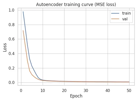
In this run, both training and validation loss drop quickly during the first epochs and then converge smoothly, with no large gap between them in the plotted curve. This suggests the model is learning a consistent reconstruction baseline for this feature space.
Outcome of This Step
At the end of training, we have a model that can reconstruct typical authentication events.
However, the model still does not output “anomaly” decisions.
To detect anomalies, we must:
- run the trained model over all events,
- compute reconstruction error per event,
- and choose a threshold to flag the most unusual cases.
That is the focus of the next step.
Step 4 — From Reconstruction Error to Anomalies (Scoring + Thresholding)
After training, the autoencoder can reconstruct typical authentication behavior.
However, it does not output anomaly labels directly.
To turn reconstruction into detection, we compute a reconstruction error score for each event and define a threshold to flag the most unusual cases.
Running Inference on the Full Dataset
We apply the trained model to the entire feature matrix (X_all_scaled).
This includes:
- the training split,
- the validation split,
- and all other events in the dataset.
model.eval()

with torch.no_grad():
    X_all_t = torch.tensor(X_all_scaled, dtype=torch.float32).to(device)
    X_hat_t = model(X_all_t)
X_hat = X_hat_t.cpu().numpy()model.eval()switches the model to inference mode.torch.no_grad()disables gradient tracking (faster and correct for inference).X_hatis the reconstructed version ofX_all_scaled.
Computing Reconstruction Error (Anomaly Score)
For each event, we compute mean squared reconstruction error across features:
recon_error = np.mean((X_hat - X_all_scaled) ** 2, axis=1)This produces a single score per event:
- low score → model reconstructs well → behavior is familiar
- high score → model reconstructs poorly → behavior deviates from learned patterns
At this stage, these are still scores — not anomaly decisions.
Inspecting the Error Distribution
Before choosing a threshold, we inspect the distribution of reconstruction error:
plt.figure(figsize=(6, 4))
sns.histplot(recon_error, bins=50, kde=True)
plt.title("Reconstruction error distribution")
plt.xlabel("Reconstruction error (MSE)")
plt.ylabel("Count")
plt.show()
In this dataset, the reconstruction errors concentrate at low values with a visible right tail. That tail is what we exploit when defining a threshold: it captures the most poorly reconstructed (i.e., most unusual) events under the learned baseline.
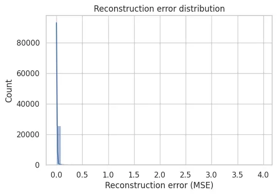
This shape is exactly what makes thresholding meaningful.
Attaching Scores Back to the Feature DataFrame
To analyze results, we attach reconstruction error back to an interpretable DataFrame.
We use the transformed feature DataFrame (X_tf) rather than the standardized version,
because it is easier to interpret feature values in human terms.
df_scores = X_tf.copy()
df_scores["recon_error"] = recon_error
Now each event has both:
- its feature values,
- and an anomaly score.
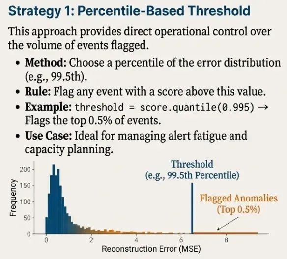
Thresholding Strategy 1: Percentile-Based Threshold
A practical and widely used thresholding approach is to flag the top X% most unusual events.
For example, using the 99.5th percentile:
p = 99.5
threshold_pct = np.percentile(recon_error, p)
threshold_pct
We flag anomalies as those exceeding the threshold:
df_scores["is_anomaly_pct"] = (df_scores["recon_error"] > threshold_pct).astype(int)
df_scores["is_anomaly_pct"].value_counts()
This approach is attractive operationally because it provides direct control over alert volume.
For example:
- 99.0 → ~1% of events flagged
- 99.5 → ~0.5% of events flagged
- 99.9 → ~0.1% of events flagged
Thresholding Strategy 2: IQR-Based Threshold (Robust Alternative)
As a second option, we can use an IQR-based rule:
threshold = Q3 + k * IQR
where IQR = Q3 - Q1.
q1, q3 = np.percentile(recon_error, [25, 75])
iqr = q3 - q1

k = 3.0
threshold_iqr = q3 + k * iqr
threshold_iqr
And flag anomalies:
df_scores["is_anomaly_iqr"] = (df_scores["recon_error"] > threshold_iqr).astype(int)
df_scores["is_anomaly_iqr"].value_counts()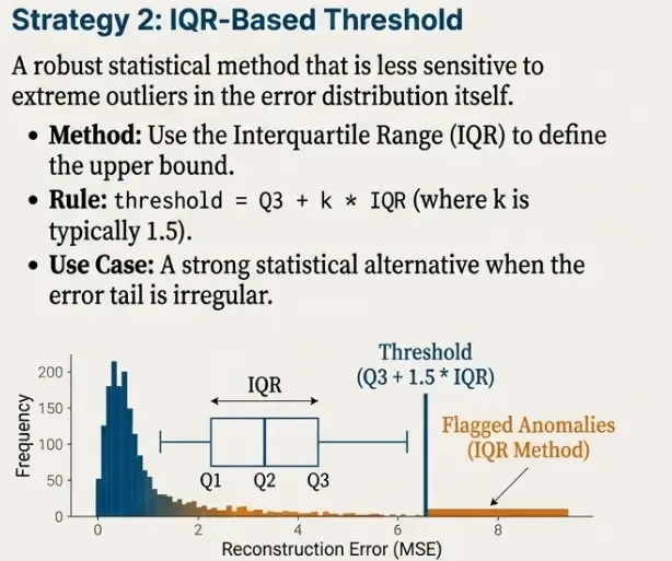
This method is less directly controllable than percentiles, but often more robust when the error distribution has irregular tails.
Inspecting Top Anomalies
Finally, we inspect the highest-scoring events:
df_scores.sort_values("recon_error", ascending=False).head(20)| index | hour | dayofweek | is_failure | user_ip_count | user_login_count | recon_error | is_anomaly_pct |
|---|---|---|---|---|---|---|---|
| 19430 | 13.0 | 1.0 | 1.0 | 4.584967 | 6.96508 | 3.972526 | 1 |
| 2296 | 0.0 | 2.0 | 0.0 | 4.574711 | 6.96508 | 1.311368 | 1 |
| 14365 | 0.0 | 2.0 | 0.0 | 4.584967 | 6.96508 | 1.269451 | 1 |
| 14377 | 0.0 | 2.0 | 0.0 | 4.584967 | 6.96508 | 1.269451 | 1 |
| 14384 | 0.0 | 2.0 | 0.0 | 4.584967 | 6.96508 | 1.269451 | 1 |
| 14370 | 0.0 | 2.0 | 0.0 | 4.584967 | 6.96508 | 1.269451 | 1 |
| 14376 | 0.0 | 2.0 | 0.0 | 4.584967 | 6.96508 | 1.269451 | 1 |
| 14363 | 0.0 | 2.0 | 0.0 | 4.584967 | 6.96508 | 1.269451 | 1 |
| 14385 | 1.0 | 2.0 | 0.0 | 4.584967 | 6.96508 | 1.111287 | 1 |
| 14393 | 1.0 | 2.0 | 0.0 | 4.584967 | 6.96508 | 1.111287 | 1 |
| 19158 | 0.0 | 1.0 | 0.0 | 4.574711 | 6.96319 | 1.093410 | 1 |
| 19155 | 0.0 | 1.0 | 0.0 | 4.574711 | 6.96319 | 1.093410 | 1 |
| 19151 | 0.0 | 1.0 | 0.0 | 4.574711 | 6.96319 | 1.093410 | 1 |
| 19136 | 0.0 | 1.0 | 0.0 | 4.574711 | 6.96319 | 1.093410 | 1 |
| 19150 | 0.0 | 1.0 | 0.0 | 4.574711 | 6.96319 | 1.093410 | 1 |
| 1136 | 0.0 | 1.0 | 0.0 | 4.574711 | 6.96319 | 1.093410 | 1 |
| 13112 | 0.0 | 1.0 | 0.0 | 4.574711 | 6.96319 | 1.093410 | 1 |
| 1112 | 0.0 | 1.0 | 0.0 | 4.574711 | 6.96319 | 1.093410 | 1 |
| 13101 | 0.0 | 1.0 | 0.0 | 4.574711 | 6.96319 | 1.093410 | 1 |
| 19163 | 0.0 | 1.0 | 0.0 | 4.574711 | 6.96319 | 1.093410 | 1 |
In this run, the top-scoring rows are driven by combinations that the model reconstructs poorly. For example, the highest anomaly includes is_failure = 1 together with high user_ip_count, while many of the other top rows correspond to off-hours logins (hour 0–1) combined with high user_ip_count.
These scores are not “attack labels”; they are triage candidates that should be investigated by joining back to the raw Elasticsearch event context (user, source IP, host, logon type, etc.).
Outcome of This Step
At the end of this scoring phase, we have:
- a trained reconstruction model,
- a continuous anomaly score per event,
- one or more thresholding strategies,
- and a set of flagged anomalous events.
This completes the full unsupervised detection workflow:
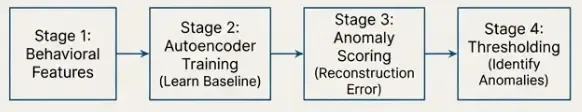
Summary
In this post, we built a complete unsupervised anomaly detection pipeline for authentication telemetry.
Starting from a compact set of behavioral features, we:
- validated and conditioned the feature space,
- trained a simple and interpretable autoencoder,
- converted reconstruction error into a continuous anomaly score,
- and applied thresholding strategies to surface rare events.
Throughout the process, several design principles guided the implementation:
- anomalies are treated as deviations, not attacks,
- failures are contextual signals, not anomalies by default,
- and model decisions are separated from operational thresholds.
The result is not a rule engine or an attack classifier, but a behavioral baseline that highlights statistically unusual authentication activity.
This kind of detector is most effective when used as an upstream signal: to reduce noise, prioritize investigations, and complement traditional security controls.
What’s Next
While autoencoders provide a strong baseline, they are not the only option for unsupervised detection.
In the next part of this series, we will compare this approach against alternative unsupervised models, including:
- distance-based methods,
- density-based techniques,
- and isolation-based detectors.
The goal is not to declare a single “best” model, but to understand the trade-offs between sensitivity, stability, interpretability, and operational cost.
From there, the series will move toward orchestration, deployment, and operationalization of these models within a real security pipeline.
Part 3: Benchmarking Unsupervised Models for Authentication Anomaly Detection
Full code available: engineering-security-ml