
Introduction
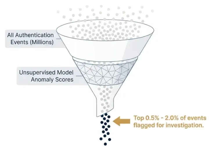
In the previous posts, we built an unsupervised detection pipeline: behavioral features from Windows authentication telemetry, then an autoencoder that converts deviations into anomaly scores.
At that point, a natural question arises:
Is this the right model?
Answering that question is harder than it seems.
In supervised machine learning, model evaluation is relatively straightforward: you compare predictions against labeled ground truth and compute metrics such as accuracy, precision, or recall.
In security anomaly detection, things are different.
- Labels are rare and noisy.
- Attacks are rare, evolving, and often subtle.
- “Unusual” does not automatically mean “malicious”.
As a result, choosing a model based on intuition, popularity, or a single demo can be dangerously misleading.
This post focuses on the third stage of the pipeline: benchmarking unsupervised models in a way that reflects SOC constraints.
What This Post Is About
This post is not about proposing a new detection algorithm. Instead, it addresses a more fundamental question:
Given several unsupervised models, how do we decide which one is appropriate for a real security use case?
To answer that, we evaluate multiple models on the same feature space, inject controlled synthetic anomalies (proxy ground truth), and compare detectors using operational metrics under an alert budget.
The goal is comparative: understand trade-offs under realistic constraints, not crown a single “best” model.
Why Benchmarking Matters More Than the Model
In practice, many security ML failures come from evaluation and thresholding choices, not algorithms. Benchmarking forces the discussion into operational terms: alert volume, missed anomalies, and stability over time.
Scope and Continuity
As in the previous posts, the focus remains on authentication telemetry. This keeps the problem well-scoped and the results interpretable.
The same principles, however, apply to richer datasets: process execution, PowerShell activity, lateral movement signals, or network telemetry.
Authentication logs serve here as a controlled baseline for understanding how unsupervised models should be evaluated before being trusted.
What Comes Next
The rest of this post will:
- Explain why benchmarking unsupervised models in security is fundamentally hard.
- Introduce synthetic anomalies as a controlled evaluation tool.
- Compare several common unsupervised detectors under the same conditions.
- And interpret the results from a security and SOC perspective.
Only after that does it make sense to talk about deployment, orchestration, and production pipelines — which is where the next part of this series will go.
The Benchmarking Problem in Unsupervised Security ML
Benchmarking machine learning models usually assumes one thing:
We can compare model outputs to reliable ground truth labels.
In supervised learning, this assumption holds. You train a model, compare predictions against labeled data, and compute metrics such as accuracy, precision, recall, or ROC curves.
In security anomaly detection, that assumption breaks almost immediately.
Why Ground Truth Is Rare (or Unreliable)
In real authentication telemetry:
- Most events are unlabeled.
Just because an authentication event was never investigated does not mean it was benign. Likewise, many investigations end without a clear conclusion. As a result, historical labels — when they exist at all — are a poor foundation for evaluating unsupervised models.
Anomaly Does Not Mean Attack
In authentication telemetry, anomaly is a statement about deviation, not intent. Benign anomalies are common, for example:
- travel, VPN, or remote-work changes,
- new devices or IP churn,
- role changes that legitimately shift login volume or hours.
Benchmarking must therefore focus on behavioral separation, not “attack detection”.
Why Traditional Metrics Are Misleading
Without reliable labels, common ML metrics lose meaning:
- Accuracy is meaningless when 99.9% of events are normal.
- ROC curves assume a well-defined positive class.
- F1-score hides operational trade-offs.
A model that flags more anomalies may look better on paper while being unusable in practice due to alert overload.
This is why unsupervised security ML requires different evaluation thinking.
Synthetic Anomalies as a Proxy Ground Truth
To evaluate models in a controlled way, we introduce synthetic anomalies.
These are not random perturbations. They are behaviorally implausible events constructed with intent.
Examples include:
- authentication events at extreme or inconsistent times,
- rare or previously unseen user–IP combinations,
- combinations of features that do not appear in normal data.
The purpose of synthetic anomalies is not to simulate attacks. It is to create known deviations against which models can be compared.
This provides a limited but useful proxy for ground truth: we know which events are intentionally abnormal.
What Synthetic Anomalies Can (and Cannot) Tell Us
Synthetic anomalies allow us to answer questions such as:
- Does the model rank abnormal behavior higher than normal behavior?
- How many anomalies are detected under a fixed alert budget?
- Which models are more sensitive or more conservative?
They do not tell us:
- whether a model detects real-world attacks,
- or how it performs against unknown adversarial behavior.
This distinction is important.
The goal is comparative evaluation, not absolute validation.
From “Best Model” to “Best Trade-Off”
Instead of asking:
Which model is best?
We ask:
Which model provides the best trade-off between sensitivity, stability, and operational cost for this use case?
Answering that question requires:
- consistent preprocessing,
- consistent evaluation rules,
- and metrics aligned with how detections are actually used.
The next section introduces the models included in this benchmark and explains why each one was chosen.
Models Under Evaluation
To benchmark unsupervised anomaly detection meaningfully, models must be evaluated under the same conditions and with a clear understanding of what each one actually does.
All models in this post operate on the same feature space, use the same preprocessing, and are evaluated using the same alert budget and metrics whenever possible.
The goal is not to exhaustively cover every algorithm, but to compare representative families of unsupervised detectors commonly used in security and anomaly detection.
Isolation Forest (IF)
Isolation Forest is based on a simple idea:
Anomalies are easier to isolate than normal points.
The model builds an ensemble of random decision trees. Points that require fewer splits to isolate are considered more anomalous.
- Works best when anomalies are globally different.
In security contexts:
- Often conservative
- Tends to miss subtle anomalies
- Useful when false positives are very costly
Isolation Forest is a common baseline: fast, robust, and often conservative.
One-Class Support Vector Machine (OC-SVM)
One-Class SVM learns a boundary that encloses normal data.
Rather than modeling anomalies directly, it answers the question: is this point outside the learned “normal” region?
Key properties:
- Learns a global decision boundary
- Produces a signed distance or anomaly score
- Sensitive to feature scaling and kernel choice
In security contexts:
- Very powerful when features are well conditioned
- Can be unstable if the feature space is noisy
- Often achieves high recall under tight alert budgets
OC-SVM can be effective in authentication telemetry, but requires careful preprocessing to avoid overfitting.
Local Outlier Factor (LOF)
Local Outlier Factor is a density-based method.
Instead of comparing points globally, it compares each point to its local neighborhood and measures how isolated it is relative to nearby points.
Key properties:
- Detects local deviations
- Produces an anomaly score
- Sensitive to neighborhood size (
n_neighbors)
In security contexts:
- Good at detecting rare behavior within common patterns
- Sensitive to noise and feature correlations
- Scores may be unstable across datasets
LOF is particularly useful when anomalies are locally rare rather than globally extreme.
Autoencoder (Reconstruction-Based)
An autoencoder is a neural network trained to reconstruct its input. The intuition is straightforward:
- normal behavior is reconstructed well,
- deviations increase reconstruction error.
Autoencoders require careful normalization and sensible capacity/regularization.
In security contexts:
- Produces smooth, continuous scores for prioritization
- Can detect subtle shifts if features are stable
- Requires drift monitoring and retraining strategy
DBSCAN (Density-Based Clustering)
DBSCAN is fundamentally different from the other models.
It is a clustering algorithm that labels points as:
- belonging to a cluster, or
- noise (outliers).
Key properties:
- Does not produce a continuous anomaly score
- Directly flags noise points
- Highly sensitive to
epsandmin_samples
In security contexts:
- Useful as a noise detector or pre-filter
- Difficult to integrate into alert budgets
- Not directly comparable to score-based models
DBSCAN is included deliberately to illustrate an important point: not all anomaly detectors are ranking-based, and evaluation strategies must adapt accordingly.
Why These Models?
These models were selected because they represent different detection philosophies:
| Family | Model |
|---|---|
| Tree-based isolation | Isolation Forest |
| Boundary learning | One-Class SVM |
| Local density | LOF |
| Reconstruction | Autoencoder |
| Density clustering | DBSCAN |
Together, they provide a broad view of how unsupervised models behave under the same behavioral data.
The next section introduces the evaluation framework used to compare these models fairly, focusing on alert budgets and operational metrics rather than abstract ML scores.
A Common Evaluation Framework
Comparing unsupervised models only makes sense if they are evaluated under a shared and realistic framework.
In security, a model is not judged solely by how well it separates data points mathematically, but by how usable its output is in practice.
This section defines the evaluation principles used throughout this benchmark.
What We Can (and Cannot) Measure
Because the problem is unsupervised, there are clear limits to what evaluation can tell us.
We cannot reliably measure:
- real attack detection rate,
- absolute accuracy,
- or long-term adversarial robustness.
We can measure:
- how models rank abnormal behavior,
- how many anomalies they surface under constraints,
- and how much noise they generate.
This benchmark focuses on what can be measured consistently.
Alert Budget: A Security-Driven Constraint
Detection systems do not operate with unlimited analyst capacity, so we evaluate models under an explicit alert budget.
We define an alert budget as:
The percentage of total events that a model is allowed to flag as anomalous.
Examples:
- 0.5% → very strict budget, minimal noise
- 1.0% → balanced operational load
- 2.0% → higher sensitivity, more analyst effort
By fixing the alert budget, we ensure that models are compared under equal operational cost, not equal mathematical thresholds.
Ranking-Based Evaluation
Most models in this benchmark produce a continuous anomaly score.
For these models:
- events are ranked by anomaly score,
- the top N% (defined by the alert budget) are flagged as anomalies,
- all other events are treated as normal.
This mirrors real usage: analysts investigate the most unusual events first.
Noise-Based Models (DBSCAN)
DBSCAN does not produce a continuous score.
Instead, it directly labels events as:
- clustered (normal),
- or noise (anomalous).
Because of this:
- DBSCAN cannot be evaluated under a fixed alert budget,
- its alert volume depends entirely on hyperparameters.
For DBSCAN, evaluation focuses on:
- how many noise points are produced,
- how many synthetic anomalies fall into noise,
- and how noisy the result is overall.
This highlights a practical limitation of clustering-based detectors in operational settings.
Confusion Matrix in an Unsupervised Context
To quantify results, we use a confusion matrix adapted to synthetic anomalies:
- True Positive (TP): synthetic anomaly correctly flagged
- False Positive (FP): normal event incorrectly flagged
- False Negative (FN): synthetic anomaly missed
- True Negative (TN): normal event correctly ignored
This does not imply that non-synthetic events are benign; it only reflects whether an event was injected for evaluation.
Metrics Used
From the confusion matrix, we derive:
- Recall: fraction of injected anomalies detected
- Precision: fraction of alerts that are injected anomalies
- False Positive Rate (FPR): fraction of normal events flagged
- Alert Rate: fraction of events sent to analysts
These metrics align directly with security concerns: missed anomalies, wasted analyst time, and operational cost.
Why Accuracy Is Not Used
Accuracy is excluded: in highly imbalanced settings, a model that flags nothing can look “accurate” while being operationally useless.
This benchmark prioritizes actionable signal over statistical comfort.
Outcome of the Framework
By fixing:
- the feature space,
- preprocessing,
- alert budgets,
- and evaluation metrics,
we ensure that observed differences between models reflect behavioral differences, not evaluation artifacts.
With the framework defined, we can move to synthetic anomaly generation and the benchmark dataset.
Synthetic Anomalies and Experimental Setup
Without reliable ground truth, we introduce a controlled reference: synthetic anomalies (intentional behavioral deviations) used for benchmarking. The objective is not attack simulation, but reproducible stress tests for different detectors.
Why Synthetic Anomalies Are Needed
Synthetic anomalies provide a controlled proxy: we know what was altered, can quantify ranking behavior, and compare detectors under identical conditions. This enables relative benchmarking, not real-world attack validation.
Design Principles for Synthetic Anomalies
To avoid unrealistic “easy outliers”, the anomalies used here follow three principles:
-
Plausibility All feature values remain within realistic ranges.
-
Subtlety Many anomalies are ambiguous, not obviously malicious.
-
Diversity Different anomaly patterns stress different detection mechanisms.
The goal is to approximate plausible deviations seen in real authentication telemetry.
Anomaly Families
Four types of synthetic anomalies are generated, with increasing severity:
| Type | Description |
|---|---|
off_hours | Logins at unusual but still plausible times |
rare_ip | Authentication from infrequently used IPs |
high_activity | Higher-than-usual authentication volume |
combined | Multiple deviations in the same event |
Each anomaly type targets a different behavioral dimension: time, frequency, recurrence, or combinations thereof.
Generating Synthetic Anomalies
Synthetic anomalies are created by sampling existing normal events and applying controlled transformations.
The implementation below is used as-is in the notebook:
def generate_synthetic_anomalies(
    X,
    n_anomalies,
    random_state=42,
):
    """
    Generate realistic authentication anomalies with different patterns
    and severities. All values remain within plausible ranges.
    """
    rng = np.random.default_rng(random_state)

    X_syn = X.sample(
        n=n_anomalies,
        replace=True,
        random_state=random_state
    ).copy()

    # Assign anomaly types
    anomaly_types = rng.choice(
        ["off_hours", "rare_ip", "high_activity", "combined"],
        size=n_anomalies,
        p=[0.35, 0.30, 0.20, 0.15],
    )
    X_syn["anomaly_type"] = anomaly_types

    # ---- Type A: off-hours login (subtle) ----
    mask = anomaly_types == "off_hours"
    X_syn.loc[mask, "hour"] = rng.choice([5, 6, 21, 22], size=mask.sum())

    # ---- Type B: rare IP usage (medium) ----
    mask = anomaly_types == "rare_ip"
    ip_low = float(X_syn["user_ip_count"].quantile(0.10))
    X_syn.loc[mask, "user_ip_count"] = ip_low * rng.uniform(0.8, 1.2, size=mask.sum())

    # ---- Type C: higher-than-usual activity (medium-high) ----
    mask = anomaly_types == "high_activity"
    mult = rng.uniform(1.15, 1.35, size=mask.sum())
    X_syn.loc[mask, "user_login_count"] = (
        X_syn.loc[mask, "user_login_count"].to_numpy() * mult
    )

    # ---- Type D: combined deviation (high severity) ----
    mask = anomaly_types == "combined"
    X_syn.loc[mask, "hour"] = rng.choice([2, 3, 4, 22, 23], size=mask.sum())

    ip_low = float(X_syn["user_ip_count"].quantile(0.10))
    X_syn.loc[mask, "user_ip_count"] = ip_low * rng.uniform(0.6, 1.0, size=mask.sum())

    mult = rng.uniform(1.30, 1.60, size=mask.sum())
    X_syn.loc[mask, "user_login_count"] = (
        X_syn.loc[mask, "user_login_count"].to_numpy() * mult
    )

    return X_syn
This function ensures that anomalies are:
- derived from real behavioral patterns,
- modified in controlled ways,
- and labeled by anomaly type for later analysis.
Injecting Anomalies Into the Dataset
Synthetic anomalies are injected at a low rate (≈1%) to reflect real-world imbalance.
Normal events are labeled with is_synthetic = 0, anomalies with is_synthetic = 1.
X_base_labeled = X_base.copy()
X_base_labeled["is_synthetic"] = 0

X_syn = generate_synthetic_anomalies(
    X_base,
    n_anomalies=int(0.01 * len(X_base)),
)

X_syn_labeled = X_syn.copy()
X_syn_labeled["is_synthetic"] = 1

df_mix = pd.concat(
    [X_base_labeled, X_syn_labeled],
    ignore_index=True
)
A quick sanity check shows the resulting class balance and anomaly mix:
df_mix["is_synthetic"].value_counts()Output:
is_synthetic
0    26417
1      264
Name: count, dtype: int64df_mix["anomaly_type"].value_counts()Output:
anomaly_type
normal           26417
off_hours           94
rare_ip             76
high_activity       61
combined            33
Name: count, dtype: int64
This distribution ensures that:
- most anomalies are subtle,
- extreme cases are rare,
- and no single pattern dominates the evaluation.
Preparing the Benchmark Dataset
The final benchmark dataset consists of:
- the standardized feature matrix (
X_mix_scaled), - a binary ground-truth label (
is_synthetic), - and a categorical breakdown (
anomaly_type).
X_mix = df_mix[FEATURE_COLUMNS].copy()
y_mix = df_mix["is_synthetic"].values

X_mix_scaled = scaler.transform(X_mix)
At this point, all models will see exactly the same data, and differences in performance can be attributed to model behavior rather than preprocessing artifacts.
What This Setup Enables
With this experimental setup, we can now answer:
- How well does each model rank synthetic anomalies?
- How many anomalies are detected under a fixed alert budget?
- Which types of anomalies each model is sensitive to?
What it does not answer:
- whether a model detects real attacks,
- or how it behaves under adversarial adaptation.
Those questions require production feedback and long-term monitoring. Next, we train/score each model under identical conditions.
Training and Scoring the Models
With the benchmark dataset defined, we apply multiple unsupervised models to the same standardized feature space and compare how they score events.
At this stage, we are not deciding alerts. We only ask:
How does each model score authentication events relative to one another?
To keep the comparison fair, all models use the same feature matrix (X_mix_scaled) and preprocessing; synthetic labels are used only for evaluation.
A Note on Scoring Conventions
Unsupervised models do not agree on what an “anomaly score” is. For consistency, we enforce:
Higher score = more anomalous
When a model’s native output follows the opposite convention, it is inverted.
This keeps ranking and alert-budget evaluation consistent across models.
Isolation Forest
Isolation Forest assigns an anomaly score based on how quickly a point is isolated in random trees.
Scikit-learn returns higher scores for more normal points, so we invert the score.
from sklearn.ensemble import IsolationForest

iforest = IsolationForest(
    n_estimators=200,
    contamination="auto",
    random_state=42
)

iforest.fit(X_mix_scaled)

scores_iforest = -iforest.score_samples(X_mix_scaled)

results_mix["score_iforest"] = scores_iforest
To understand how well the model separates normal and synthetic events, we inspect the score distribution:
plot_score_distribution(
    scores_iforest,
    y_mix,
    "Isolation Forest — anomaly score distribution"
)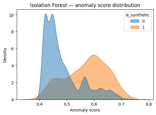
This visualization shows how much overlap exists between normal behavior and injected anomalies, which directly affects achievable recall under tight alert budgets.
One-Class SVM
One-Class SVM learns a boundary enclosing normal behavior.
Points far outside this boundary receive large negative decision values. We invert them so that higher values indicate greater deviation.
from sklearn.svm import OneClassSVM

ocsvm = OneClassSVM(
    kernel="rbf",
    gamma="scale",
    nu=0.01
)

ocsvm.fit(X_mix_scaled)

scores_ocsvm = -ocsvm.decision_function(X_mix_scaled)

results_mix["score_ocsvm"] = scores_ocsvm
Score distribution:
plot_score_distribution(
    scores_ocsvm,
    y_mix,
    "One-Class SVM — anomaly score distribution"
)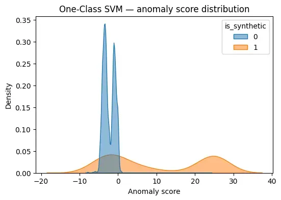
OC-SVM often produces strong separation when the feature space is well conditioned, but can also be sensitive to scaling and noise.
Local Outlier Factor (LOF)
LOF compares the local density of each point to its neighbors.
We use the negative outlier factor and invert it so that higher values indicate anomalies.
from sklearn.neighbors import LocalOutlierFactor

lof = LocalOutlierFactor(
    n_neighbors=35,
    novelty=True
)

lof.fit(X_mix_scaled)

scores_lof = -lof.score_samples(X_mix_scaled)

results_mix["score_lof"] = scores_lof
Score distribution:
plot_score_distribution(
    scores_lof,
    y_mix,
    "Local Outlier Factor — anomaly score distribution"
)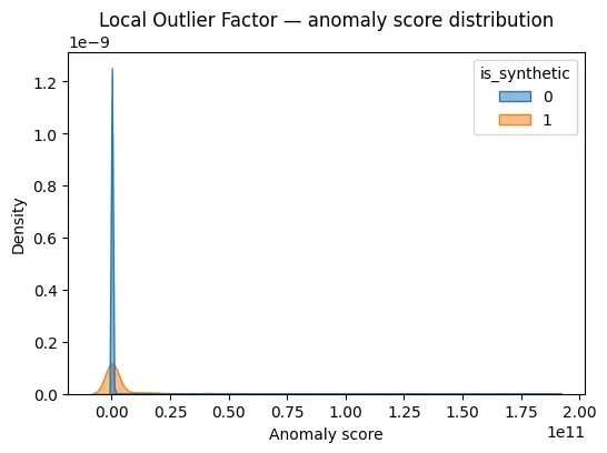
LOF is particularly sensitive to local deviations, which makes it useful for certain anomaly types but unstable in others.
Autoencoder (Reconstruction Error)
The autoencoder trained in Part 2 is reused here without retraining.
Anomaly score is defined as mean squared reconstruction error.
import torch

model.eval()

with torch.no_grad():
    X_t = torch.tensor(X_mix_scaled, dtype=torch.float32).to(device)
    X_hat = model(X_t).cpu().numpy()

scores_autoencoder = ((X_hat - X_mix_scaled) ** 2).mean(axis=1)

results_mix["score_autoencoder"] = scores_autoencoder
Score distribution:
plot_score_distribution(
    scores_autoencoder,
    y_mix,
    "Autoencoder — reconstruction error distribution"
)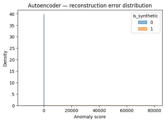
Reconstruction-based models tend to produce smooth score distributions, which can be advantageous for thresholding and alert prioritization.
DBSCAN (Noise-Based Detection)
DBSCAN does not produce a continuous anomaly score.
Instead, it labels each point as either:
- part of a dense cluster, or
- noise (
-1).
Noise points are treated as anomalies.
from sklearn.cluster import DBSCAN

dbscan = DBSCAN(
    eps=0.8,
    min_samples=25
)

labels = dbscan.fit_predict(X_mix_scaled)

results_mix["is_anomaly_dbscan"] = (labels == -1).astype(int)
results_mix["dbscan_cluster"] = labels
Because DBSCAN is not ranking-based:
- it cannot be evaluated under an alert budget,
- its alert volume depends entirely on hyperparameters.
This limitation will be important when interpreting results.
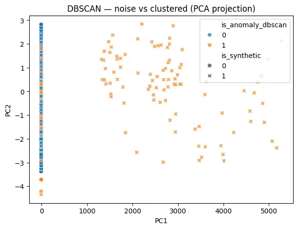
PCA is used here purely for visualization, projecting the high-dimensional feature space into two dimensions so that DBSCAN’s clustering and noise behavior can be inspected by a human.
from sklearn.decomposition import PCA

pca = PCA(n_components=2, random_state=42)
X_2d = pca.fit_transform(X_mix_scaled)

plt.figure(figsize=(7, 5))
sns.scatterplot(
    x=X_2d[:, 0],
    y=X_2d[:, 1],
    hue=results_mix["is_anomaly_dbscan"],
    style=results_mix["is_synthetic"],
    alpha=0.7
)
plt.title("DBSCAN — noise vs clustered (PCA projection)")
plt.xlabel("PC1")
plt.ylabel("PC2")
plt.show()
This projection shows how DBSCAN separates dense behavioral regions from sparse points: noise points lie outside well-defined clusters, but lack any ranking or notion of severity, making DBSCAN unsuitable for alert prioritization despite its ability to flag structural outliers.
Summary of Scoring Outputs
At the end of this step, results_mix contains:
-
continuous anomaly scores for:
- Isolation Forest
- One-Class SVM
- LOF
- Autoencoder
-
binary anomaly labels for:
- DBSCAN
-
ground-truth labels:
is_syntheticanomaly_type
All subsequent evaluation uses only these outputs (no retraining). Next, we translate scores into decisions under an alert budget.
Alert Budgets and Recall-Based Evaluation
At this point, each model has produced either:
- a continuous anomaly score (Isolation Forest, OC-SVM, LOF, Autoencoder), or
- a binary noise label (DBSCAN).
Raw scores alone are not actionable. The key operational constraint is:
How many alerts can realistically be investigated?
This is where alert budgets become central.
What Is an Alert Budget?
An alert budget defines the fraction of total events that a detection system is allowed to flag for investigation.
Examples:
- 0.5% → very strict, minimal noise
- 1.0% → balanced, common SOC target
- 2.0% → higher sensitivity, higher analyst cost
Instead of comparing models at arbitrary thresholds, we compare them under the same operational cost.
This avoids a common pitfall in anomaly detection benchmarking: models that look “better” simply because they generate more alerts.
Recall at Fixed Budget
To evaluate models fairly, we use recall at budget:
Given a fixed alert budget, what fraction of injected anomalies are captured?
This directly answers: if I can only review X% of events, how many injected anomalies appear in that set?
Computing Recall at Budget
The following helper function implements this logic:
def recall_at_budget(scores, y_true, budget_pct):
    scores = np.asarray(scores)
    y_true = np.asarray(y_true).astype(int)

    thr = np.percentile(scores, 100 - budget_pct)
    y_pred = (scores >= thr).astype(int)

    captured = ((y_pred == 1) & (y_true == 1)).sum()
    total_anomalies = y_true.sum()

    recall = captured / (total_anomalies + 1e-12)

    return recall, y_pred.sum(), captured, thr
This function:
- ranks events by anomaly score,
- selects the top budget_pct percent,
- computes how many synthetic anomalies fall within that set.
Recall vs Alert Budget (Global)
We now evaluate all score-based models across multiple budgets:
budgets = [0.5, 1.0, 2.0]
rows = []

model_scores = {
    "iforest": results_mix["score_iforest"].values,
    "ocsvm": results_mix["score_ocsvm"].values,
    "lof": results_mix["score_lof"].values,
    "autoencoder": results_mix["score_autoencoder"].values,
}

for model, scores in model_scores.items():
    for b in budgets:
        r, selected, captured, thr = recall_at_budget(scores, y_mix, b)
        rows.append({
            "model": model,
            "budget_pct": b,
            "recall": r,
            "selected": selected,
            "captured": captured,
            "threshold": thr,
        })

df_budget = pd.DataFrame(rows)
df_budget
Visualization:
plt.figure(figsize=(7, 4))
sns.lineplot(
    data=df_budget,
    x="budget_pct",
    y="recall",
    hue="model",
    marker="o"
)
plt.title("Recall vs Alert Budget")
plt.xlabel("Alert budget (% of events reviewed)")
plt.ylabel("Recall of synthetic anomalies")
plt.ylim(0, 1.05)
plt.show()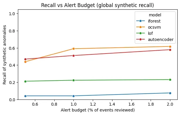
How to Read This Plot
This plot reveals trade-offs:
- Steep curves → models that quickly capture anomalies but may be noisy
- Flat curves → conservative models that miss subtle deviations
- Crossings → models that dominate only under specific budgets
This is exactly the kind of information required to choose a detector for a real SOC.
Confusion-Matrix–Based Evaluation at a Fixed Alert Budget
To compare models operationally, we translate scores into binary decisions under a fixed alert budget and compute confusion-matrix metrics.
From Scores to Decisions Under an Alert Budget
For score-based models (Isolation Forest, OC-SVM, LOF, Autoencoder), evaluation is consistent: rank by score and flag only the top N% (the alert budget).
In this experiment, we fix the alert budget to 1%, meaning that at most 1% of all authentication events would be reviewed by analysts.
The following helper function implements this logic:
def confusion_metrics(scores, y_true, budget_pct):
    scores = np.asarray(scores)
    y_true = np.asarray(y_true).astype(int)

    thr = np.percentile(scores, 100 - budget_pct)
    y_pred = (scores >= thr).astype(int)

    tp = ((y_pred == 1) & (y_true == 1)).sum()
    fp = ((y_pred == 1) & (y_true == 0)).sum()
    tn = ((y_pred == 0) & (y_true == 0)).sum()
    fn = ((y_pred == 0) & (y_true == 1)).sum()

    precision = tp / (tp + fp + 1e-12)
    recall = tp / (tp + fn + 1e-12)
    fpr = fp / (fp + tn + 1e-12)

    return {
        "tp": tp, "fp": fp, "tn": tn, "fn": fn,
        "precision": precision,
        "recall": recall,
        "fpr": fpr,
        "threshold": thr
    }
This converts continuous anomaly scores into a binary alert decision, making models directly comparable.
Metrics Used
Each model is evaluated using the following metrics:
-
True Positives (TP) Synthetic anomalies correctly detected.
-
False Positives (FP) Normal events incorrectly flagged.
-
False Negatives (FN) Synthetic anomalies missed by the model.
-
Precision Of all alerts raised, how many were truly anomalous?
-
Recall Of all injected anomalies, how many were detected?
-
False Positive Rate (FPR) How much normal behavior is disrupted?
These metrics are far more meaningful for security operations than accuracy or ROC curves.
Results at 1% Alert Budget
At a fixed 1% alert budget, the results are:
| model | budget_pct | tp | fp | tn | fn | precision | recall | fpr | threshold |
|---|---|---|---|---|---|---|---|---|---|
| ocsvm | 1.0 | 156 | 114 | 26303 | 108 | 0.5778 | 0.5909 | 0.0043 | 0.5079 |
| autoencoder | 1.0 | 135 | 142 | 26275 | 129 | 0.4874 | 0.5114 | 0.0054 | 0.4081 |
| lof | 1.0 | 59 | 216 | 26201 | 205 | 0.2145 | 0.2235 | 0.0082 | 1.07e9 |
| iforest | 1.0 | 11 | 262 | 26155 | 253 | 0.0403 | 0.0417 | 0.0099 | 0.6855 |
| dbscan | — | 151 | 32 | 26385 | 113 | 0.8251 | 0.5720 | 0.0012 | noise-based |
How to Interpret These Results
Several important insights emerge:
- OC-SVM achieves the highest recall among score-based models, capturing the largest fraction of synthetic anomalies under the same alert budget.
- Autoencoders provide a strong balance between recall and stability, with smooth scoring behavior.
- LOF and Isolation Forest are significantly more conservative, missing most injected anomalies.
- DBSCAN performs well in precision but is fundamentally different:
- it does not obey an alert budget,
- its alert volume is driven entirely by density parameters.
Model choice depends on whether you prioritize recall, precision, alert control, or stability over time.
Recall by Anomaly Type
So far, recall was computed globally, across all synthetic anomalies.
But not all anomalies are the same.
In this benchmark, injected anomalies are labeled by behavioral category:
off_hoursrare_iphigh_activitycombined
A model that performs well globally may still fail completely on certain anomaly types.
Why Per-Type Recall Matters
Different models are sensitive to different kinds of deviations:
- global vs local
- temporal vs frequency-based
- isolated vs combined signals
Evaluating recall by anomaly type reveals what a model is actually good at.
Computing Recall per Anomaly Type
rows = []

for model, scores in model_scores.items():
    for b in budgets:
        thr = np.percentile(scores, 100 - b)
        y_pred = (scores >= thr).astype(int)

        for atype in df_mix["anomaly_type"].unique():
            if atype == "normal":
                continue

            mask = (df_mix["anomaly_type"] == atype).values
            total = mask.sum()
            captured = ((y_pred == 1) & mask).sum()
            recall = captured / (total + 1e-12)

            rows.append({
                "model": model,
                "budget_pct": b,
                "anomaly_type": atype,
                "recall": recall,
                "total": total,
                "captured": captured,
            })

df_budget_by_type = pd.DataFrame(rows)
df_budget_by_type
Visualization as a heatmap (for a fixed budget):
budget = 1.0

pivot = (
    df_budget_by_type[df_budget_by_type["budget_pct"] == budget]
    .pivot(index="model", columns="anomaly_type", values="recall")
)

plt.figure(figsize=(7, 4))
sns.heatmap(
    pivot,
    annot=True,
    cmap="viridis",
    vmin=0,
    vmax=1
)
plt.title(f"Recall by Anomaly Type (Budget = {budget}%)")
plt.xlabel("Anomaly type")
plt.ylabel("Model")
plt.show()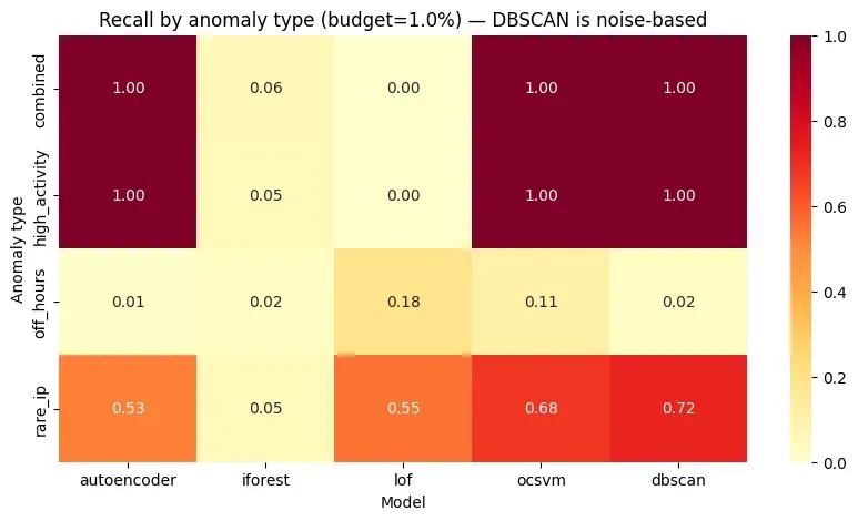
Interpreting the Heatmap
This heatmap is often the most actionable result: it shows which anomaly families each model captures (or misses) under the same budget, exposing blind spots hidden by global averages.
What These Results Actually Tell Us
At this stage, the benchmark provides operational answers (early surfacing, noise, specialization by anomaly type, robustness under budgets). It does not establish real attack detection. Instead, it tells us:
How different unsupervised detectors behave when forced to operate like real security systems.
Transition to Conclusions
The final section ties these results together and gives a practical model-selection checklist based on analyst capacity and detection goals.
Conclusions: Choosing an Unsupervised Model in Practice
After benchmarking multiple unsupervised models under the same conditions, one conclusion becomes clear:
There is no universally “best” anomaly detection model.
What exists instead are trade-offs.
Each model encodes a different assumption about what “abnormal” means, and those assumptions interact directly with:
- the feature space,
- the alert budget,
- and the types of deviations we care about.
This is precisely why benchmarking matters more than algorithm choice.
What the Benchmark Actually Demonstrates
This benchmark does not prove that any model detects real attacks.
What it demonstrates is something more practical and more honest:
- how models rank abnormal behavior,
- how quickly they surface injected deviations,
- how noisy their alerts are under realistic constraints,
- and which kinds of anomalies they are structurally good or bad at detecting.
These are the properties that determine whether a model is usable in production.
Key Observations Across Models
From the experiments, several consistent patterns emerge.
Isolation Forest
- Conservative by design
- Low false positives
- Misses subtle or contextual anomalies
Best suited for: Environments where false positives are extremely costly and only strong deviations matter.
One-Class SVM
- Very strong recall under tight alert budgets
- Sensitive to preprocessing and scaling
- Can overfit if the feature space is noisy
Best suited for: Well-conditioned behavioral features and environments prioritizing sensitivity.
Local Outlier Factor (LOF)
- Strong at detecting local deviations
- Performance varies significantly by anomaly type
- Sensitive to neighborhood size and density assumptions
Best suited for: Scenarios where anomalies are rare relative to local behavior, not globally extreme.
Autoencoder
- Smooth, stable anomaly scores
- Good balance between recall and precision
- Learns behavioral structure rather than explicit boundaries
Best suited for: Behavioral baselining and continuous anomaly scoring pipelines.
DBSCAN
- High precision for extreme outliers
- No ranking or budget control
- Highly parameter-sensitive
Best suited for: Noise detection, pre-filtering, or exploratory analysis — not primary alerting.
Why Alert Budgets Matter More Than Scores
A key takeaway is that alert budget dominates evaluation: models with similar score distributions can behave very differently once constrained by analyst capacity. Metrics that ignore this constraint (e.g., accuracy or unconstrained curves) can be misleading.
Synthetic Anomalies: A Tool, Not a Truth
The synthetic anomalies used here are not attacks. They provide relative insight into ranking behavior and blind spots under controlled conditions, not absolute proof of real-world detection.
How to Choose a Model in a Real Pipeline
Rather than selecting a model upfront, a more reliable approach is:
- Start with feature quality (bad features make every model bad).
- Benchmark multiple models early (prefer comparative behavior over intuition).
- Fix the alert budget before tuning (operational cost first).
- Evaluate by anomaly family (global metrics hide blind spots).
In practice, production systems often combine detectors and rely on correlation rather than single-model alerts.
What This Series Has Shown So Far
Across the series, we built features, trained an unsupervised baseline, and benchmarked detectors under realistic constraints—without relying on perfect labels.
What Comes Next
With benchmarking in place, the next natural steps are no longer purely ML-related.
They involve engineering:
- orchestration and retraining strategies,
- model lifecycle management,
- drift detection,
- and integration into real SOC workflows.

The next part of this series will focus on: from models to pipelines — how to operationalize these detectors in a real security environment.
Part 4: From Models to Pipelines — Operationalizing Unsupervised Detection in Security Systems
Full code available: engineering-security-ml