
Introduction
Authentication telemetry is one of the most valuable — and most challenging — data sources in security. Windows Event Logs provide detailed visibility into how users authenticate, but at scale they quickly become noisy and repetitive.
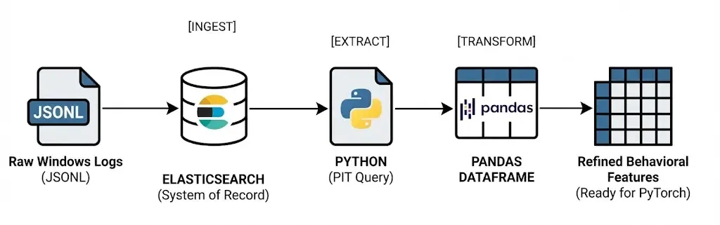
In this post, I describe the first stage of an Elastic + ML pipeline:
how to take Windows Security Event Logs, ingest them into Elasticsearch, and transform raw login events into behavioral features suitable for anomaly detection.
This post focuses on:
- Infrastructure and local development setup.
- Extracting authentication events from Elasticsearch.
- Exploratory analysis and feature engineering.
Model training will be covered in the next part.
Scope of the Dataset
Windows Security Event Logs contain many event types.
To keep the problem focused and well-defined, this first iteration works only with authentication-related events, such as:
- Successful logons (
4624). - Failed logons (
4625). - Logoff events (
4634). - Different logon types (interactive, network, remote, etc.).
In later parts of this series, this scope will be expanded to include:
- Process creation.
- Service activity.
- Lateral movement indicators.
For now, the goal is to understand how users normally authenticate.
Infrastructure Setup (Elasticsearch + Kibana)
Before diving into the pipeline, it is worth briefly clarifying what the ELK stack is and why it fits this use case so well.
The ELK stack refers to a set of components designed to ingest, store, search, and analyze large volumes of event-based data:
- Elasticsearch provides a distributed, time-oriented data store optimized for logs and events.
- Logstash (or other ingest mechanisms such as Beats or Elastic Agent) is responsible for collecting, parsing, and enriching data before it is indexed.
- Kibana sits on top of Elasticsearch and enables exploration, validation, and visualization of that data.
In this project, ELK plays a very specific role:
- Elasticsearch acts as the system of record for Windows Event Logs.
- It allows efficient filtering, aggregation, and time-based queries over authentication events.
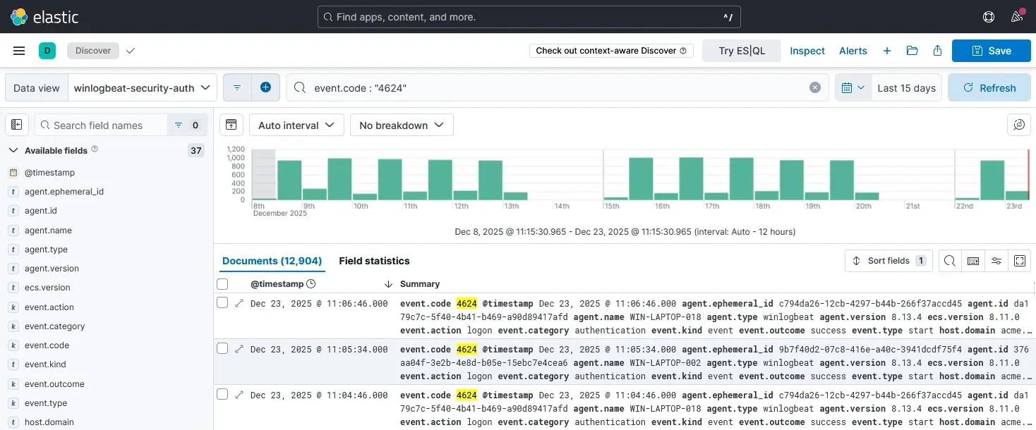
- Kibana is used to validate ingestion, inspect raw events, and later visualize anomalies.
This separation of concerns is intentional. Elasticsearch is responsible for scalable storage and retrieval, while all data science and machine learning work is performed externally in Python. This mirrors how Elastic is commonly used in real-world security and observability pipelines.
Docker Compose
The entire stack runs locally using Docker Compose.
Only the core services are deployed — all data science work happens outside containers.
services:
  elasticsearch:
    image: docker.elastic.co/elasticsearch/elasticsearch:8.18.0
    environment:
      - discovery.type=single-node
      - ES_JAVA_OPTS=-Xms2g -Xmx2g
      - xpack.security.enabled=false
    ports:
      - "9200:9200"

  kibana:
    image: docker.elastic.co/kibana/kibana:8.18.0
    environment:
      - ELASTICSEARCH_HOSTS=http://elasticsearch:9200
      - XPACK_SECURITY_ENABLED=false
    ports:
      - "5601:5601"
This setup provides:
- a single-node Elasticsearch cluster.
- Kibana for validation and exploration.
- minimal friction for local experimentation.
Development Environment (Python + uv)
All data science and machine learning work is performed locally in Python, outside of Docker.
To manage dependencies and execution, I use uv, a modern Python packaging and runtime tool.
uv provides:
- fast dependency resolution.
- isolated virtual environments.
- a single, consistent interface for running Python code.
This makes it particularly well suited for data science workflows that combine notebooks, scripts, and ML libraries.
Initializing the Project
The project is initialized with a minimal Python configuration:
uv initThis creates a pyproject.toml file, which becomes the single source of truth for:
- Python version.
- Dependencies.
- Tooling configuration.
No virtual environment needs to be created manually — uv manages it automatically.
Managing Dependencies
Dependencies are added incrementally as the project evolves:
uv add elasticsearch pandas numpy torch jupyterThis approach encourages explicit dependency management and avoids hidden system-level assumptions.
The resulting environment includes:
elasticsearchfor interacting with Elasticsearch APIspandasandnumpyfor data manipulation and analysistorchfor machine learning modelsjupyterfor exploratory analysis and experimentation
All dependencies are locked and resolved by uv, ensuring reproducibility across machines.
Running Code with uv
All Python commands are executed through uv, which guarantees they run inside the project’s managed environment.
For example, bulk ingestion scripts are executed as:
uv run python scripts/bulk_index_jsonl.py \
  --file data/winlogbeat-security-auth.jsonl \
  --index winlogbeat-security-auth-000001
This eliminates ambiguity around Python versions or active virtual environments and keeps the development workflow consistent.
Ingesting Windows Authentication Logs
In Elasticsearch, data is stored in indices.
An index can be thought of as a logical collection of documents that share a similar structure — roughly equivalent to a table in a relational database, but optimized for time-based event data.
In this pipeline, authentication events are stored in a dedicated index:
winlogbeat-security-auth-000001
Using a dedicated index allows us to:
- Isolate authentication telemetry from other event types.
- Control mappings and ingestion behavior.
- Query and analyze login activity independently.
How Indices Are Created
Elasticsearch can create indices automatically on first write, but relying on implicit creation often leads to subtle issues (unexpected mappings, data streams, or ingestion errors).
For this reason, the index is created explicitly before ingestion, with mappings suitable for Windows authentication logs.
At a high level, this index is designed to store:
- timestamped events
- ECS-compliant fields (
user,host,source,event) - flexible authentication metadata (
winlog.event_data)
This mirrors how Winlogbeat creates indices in production environments, while keeping full control over the schema.
How the Data Is Ingested
In a real-world deployment, Windows Event Logs would typically be collected and shipped using Winlogbeat or the Elastic Agent, which handle:
- log collection on endpoints
- ECS normalization
- reliable delivery to Elasticsearch
In this project, the ingestion logic is implemented manually to keep the pipeline explicit and reproducible.
Authentication events are indexed directly via the Elasticsearch API using a bulk ingestion script.
From Elasticsearch’s point of view, the resulting documents are indistinguishable from those produced by Winlogbeat.
Index Creation and Controlled Mappings
Before ingesting any data, the target index is created explicitly.
Although Elasticsearch can create indices automatically on first write, doing so often leads to unexpected mappings and ingestion errors — especially when working with structured logs such as Windows Event Logs.
To avoid this, the index is created ahead of time using a small Python script:
from elasticsearch import Elasticsearch
import os

es = Elasticsearch("http://localhost:9200")
INDEX = os.getenv("INDEX_NAME", "logs-windows.security-synth-000001")
MAPPINGS = {
    "mappings": {
        "dynamic": True,
        "properties": {
            "@timestamp": {"type": "date"},
            "source.ip": {"type": "ip"},
            "event.code": {"type": "keyword"},
            "event.action": {"type": "keyword"},
            "event.outcome": {"type": "keyword"},
            "event.category": {"type": "keyword"},
            "event.type": {"type": "keyword"},
            "user.name": {"type": "keyword"},
            "user.domain": {"type": "keyword"},
            "host.name": {"type": "keyword"},
            "host.hostname": {"type": "keyword"},
            "winlog.channel": {"type": "keyword"},
            "winlog.provider_name": {"type": "keyword"},
            "winlog.computer_name": {"type": "keyword"},
            "winlog.event_id": {"type": "long"},
            "winlog.record_id": {"type": "long"},
            "winlog.event_data": {"type": "flattened"},
            "tags": {"type": "keyword"},
        }
    }
}

if not es.indices.exists(index=INDEX):
    es.indices.create(index=INDEX, body=MAPPINGS)
The full mapping defines the expected structure of authentication events and closely follows the schema produced by Winlogbeat.
Key design decisions include:
-
Explicit types for common ECS fields Fields such as
@timestamp,source.ip,user.name, andevent.codeare mapped explicitly to ensure correct querying and aggregation behavior. -
Use of
flattenedforwinlog.event_dataWindows authentication events contain a large and variable set of key–value pairs. Mapping this field asflattenedprevents mapping explosions while preserving searchability.
This approach mirrors how Winlogbeat structures Windows Event Log indices in production, while keeping full control over the schema.
Bulk Ingestion via the Elasticsearch API
Once the index exists, authentication events are ingested using Elasticsearch’s Bulk API.
Instead of sending documents one by one, events are streamed from a JSONL file and indexed in batches. This approach is significantly more efficient and reflects how ingestion pipelines operate at scale.
The ingestion logic is implemented in a standalone script that:
- Reads authentication events line by line.
- Parses each event as a JSON document.
- Sends events to Elasticsearch in bulk batches.
- Reports indexing success and errors.
Conceptually, the ingestion flow looks like this:
JSONL file → Bulk API → Elasticsearch indexA version of the bulk action generator looks like:
#!/usr/bin/env python3
import os
import json
from elasticsearch import Elasticsearch, helpers

ES_URL = os.getenv("ELASTICSEARCH_URL", "http://localhost:9200")
ES_USER = os.getenv("ELASTIC_USERNAME", "elastic")
ES_PASS = os.getenv("ELASTIC_PASSWORD", "changeme")


def bulk_index_jsonl(path: str, index: str, chunk_size: int = 2000):
    es = Elasticsearch(
        ES_URL,
        basic_auth=(ES_USER, ES_PASS),
    ).options(request_timeout=60)

    def gen_actions():
        with open(path, "r", encoding="utf-8") as f:
            for line_no, line in enumerate(f, start=1):
                line = line.strip()
                if not line:
                    continue
                try:
                    doc = json.loads(line)
                except json.JSONDecodeError as e:
                    raise RuntimeError(f"Invalid JSON at line {line_no}: {e}") from e

                yield {
                    "_op_type": "index",
                    "_index": index,
                    "_source": doc,
                }

    ok, errors = helpers.bulk(
        es,
        gen_actions(),
        chunk_size=chunk_size,
        raise_on_error=False,
        raise_on_exception=False,
    )

    print(f"Bulk finished → indexed_ok={ok}, errors={len(errors)}")

    if errors:
        print("First error example:")
        print(json.dumps(errors[0], indent=2))


if __name__ == "__main__":
    import argparse

    p = argparse.ArgumentParser()
    p.add_argument("--file", required=True, help="Path to JSONL file")
    p.add_argument("--index", required=True, help="Target index name (NOT a data stream)")
    p.add_argument("--chunk-size", type=int, default=2000)
    args = p.parse_args()

    bulk_index_jsonl(args.file, args.index, args.chunk_size)
Using _op_type: index ensures compatibility with standard indices and avoids the constraints imposed by data streams.
Running the Ingestion Pipeline
With the index created, ingestion becomes a single command:
uv run python scripts/bulk_index_jsonl.py \
  --file data/winlogbeat-security-auth.jsonl \
  --index winlogbeat-security-auth-000001
This step produces immediate feedback on how many events were indexed successfully and whether any documents failed validation.
At this point, authentication telemetry is fully stored in Elasticsearch, and the system is ready for exploration and analysis.
From here onward, Elasticsearch is treated as the single source of truth, while all feature extraction and modeling happens externally in Python.
Example Document Structure
Each document stored in the index represents a single authentication event and follows the ECS structure used by Winlogbeat:
{
  "@timestamp": "2025-01-12T08:43:21Z",
  "event": {
    "code": "4624",
    "outcome": "success"
  },
  "user": {
    "name": "jdoe",
    "domain": "CORP"
  },
  "source": {
    "ip": "10.0.1.34"
  },
  "winlog": {
    "event_data": {
      "LogonType": "3"
    }
  }
}
This structure preserves the full context of each authentication while remaining flexible enough for downstream analysis.
Verifying Ingestion
Once ingestion is complete, the index can be validated directly:
curl -s http://localhost:9200/winlogbeat-security-auth-synth-000001/_count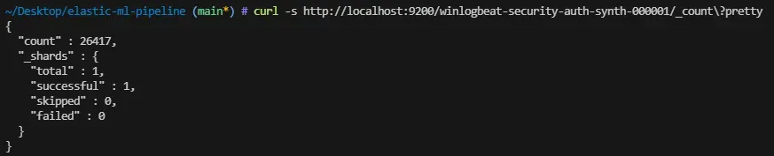
At this point, Elasticsearch becomes the single source of truth for all further analysis, exploration, and feature extraction.
Extracting Data from Elasticsearch
To retrieve authentication events efficiently and safely, I query Elasticsearch using Point-in-Time (PIT) together with search_after. This avoids deep pagination issues and guarantees a consistent view of the data, even for large indices.
This pattern is preferred over naive approaches such as increasing the size parameter or using from offsets.
Conceptually, the data flow is straightforward:
Elasticsearch → Pandas DataFrame
Opening a Point-in-Time Context
The first step is to open a Point-in-Time (PIT) against the authentication index:
pit_id = es.open_point_in_time(
    index="winlogbeat-security-auth-000001",
    keep_alive="1m"
)["id"]
This creates a stable snapshot of the index that can be queried repeatedly without being affected by concurrent writes.
Querying with search_after
Documents are retrieved in sorted batches using search_after. Each request returns a fixed number of events and provides a cursor for the next batch.
A simplified version of the query looks like this:
query = {
    "size": 2000,
    "sort": [
        {"@timestamp": "asc"},
        {"_shard_doc": "asc"}
    ],
    "pit": {
        "id": pit_id,
        "keep_alive": "1m"
    }
}
Sorting by @timestamp ensures a chronological view of authentication activity, while _shard_doc provides a deterministic tie-breaker.
Fetching Only Relevant Fields
To reduce payload size and keep the analysis focused, only authentication-related fields are retrieved:
query["_source"] = [
    "@timestamp",
    "event.code",
    "event.outcome",
    "user",
    "source",
    "winlog.event_data.LogonType"
]
These fields provide enough context to analyze:
- When authentication occurs.
- Who is authenticating.
- From where.
- And whether the attempt succeeded or failed.
Iterating and Building a DataFrame
Each batch of results is appended to an in-memory list and later converted into a Pandas DataFrame:
docs = []

while True:
    res = es.search(body=query)
    hits = res["hits"]["hits"]

    if not hits:
        break

    for h in hits:
        docs.append(h["_source"])

    query["search_after"] = hits[-1]["sort"]
Once all batches are retrieved, the PIT is closed and the raw event list is materialized as a DataFrame:
df = pd.DataFrame(docs)At this point, the DataFrame still closely resembles the original ECS documents stored in Elasticsearch.
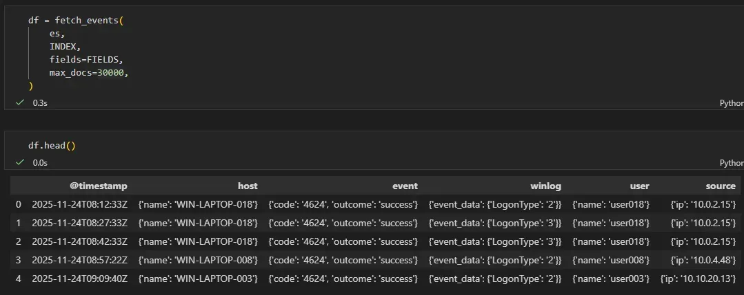
Resulting Dataset
The resulting dataset contains one row per authentication event, with nested ECS fields preserved. This makes it suitable for:
- exploratory analysis
- feature engineering
- joining back anomalies with raw context later on
The transformation into numerical features is performed in the next step.
From Raw Events to Behavioral Features
Raw ECS events are not suitable for ML models directly.
The key step is transforming authentication logs into numerical behavioral signals that capture how users authenticate, not just that they did.
At this stage, the dataset still closely resembles the original Elasticsearch documents, including nested ECS fields such as user, source, and event.
Flattening ECS Fields
Before deriving features, relevant ECS fields are flattened into explicit columns. This avoids working with nested dictionaries during analysis.
df["@timestamp"] = pd.to_datetime(df["@timestamp"], utc=True)

df["user_name"] = df["user"].apply(
    lambda x: x.get("name") if isinstance(x, dict) else None
)

df["source_ip"] = df["source"].apply(
    lambda x: x.get("ip") if isinstance(x, dict) else None
)
This step creates stable identifiers that can be safely used for grouping and aggregation.
Temporal Context
Authentication behavior is highly time-dependent. Two simple features capture most of this structure:
hour: hour of daydayofweek: day of week
df["hour"] = df["@timestamp"].dt.hour
df["dayofweek"] = df["@timestamp"].dt.dayofweek
These features allow the model to learn regular work patterns and detect off-hours activity.
Authentication Outcome
Windows authentication events encode success and failure via event codes. These are reduced to a single binary signal:
df["event_code"] = df["event"].apply(
    lambda x: x.get("code") if isinstance(x, dict) else None
)

df["is_failure"] = (df["event_code"] == "4625").astype(int)
Failures are rare, but even a small number of unexpected failures can be a strong anomaly indicator.
User-Level Behavioral Baselines
To model normal behavior, it is important to capture how active each user typically is.
A simple per-user baseline is derived by counting authentication events:
df["user_login_count"] = (
    df.groupby("user_name")["user_name"]
      .transform("count")
)
This provides a coarse measure of expected activity volume for each user.
IP Novelty per User
One of the most informative signals for authentication anomalies is IP novelty.
To capture this, a combined user–IP key is constructed:
df["user_ip"] = df["user_name"] + "_" + df["source_ip"]

df["user_ip_count"] = (
    df.groupby("user_ip")["user_ip"]
      .transform("count")
)
Low values of user_ip_count correspond to rare or previously unseen IP addresses for a given user.
Resulting Feature Set
After feature extraction, each authentication event is represented by a compact numerical vector capturing:
- temporal context (
hour,dayofweek) - authentication outcome (
is_failure) - per-user activity baselines (
user_login_count) - IP novelty (
user_ip_count)
Raw ECS fields are preserved separately for interpretability, while only numerical features are used as input to machine learning models.
This representation forms the foundation for unsupervised anomaly detection in the next stage of the pipeline.
Separating Analysis from Model Input
A deliberate design decision in this pipeline is to maintain two distinct representations of the data.
1. Raw Analysis DataFrame
The raw DataFrame preserves the full ECS context retrieved from Elasticsearch, including nested fields such as user, source, and event.
This representation is used for:
- exploratory analysis
- manual inspection of anomalies
- explaining alerts to analysts
- correlating anomalous scores with original events
Conceptually:
df_raw = df.copy()No information is lost at this stage.
2. Model Feature Matrix
Machine learning models operate on numerical vectors, not structured event documents. For this reason, a second representation is derived, containing only numerical behavioral features:
FEATURE_COLUMNS = [
    "hour",
    "dayofweek",
    "is_failure",
    "user_login_count",
    "user_ip_count",
]

X = df[FEATURE_COLUMNS].astype(float)
This matrix is the only input used for training and inference.
Why This Separation Matters
This separation provides several important benefits:
-
Explainability Anomalies detected by the model can always be traced back to the original ECS events.
-
Flexibility Features can evolve independently without re-ingesting or mutating raw data.
-
Clean ML boundaries The model never sees identifiers such as usernames or IP addresses directly.
This pattern mirrors how ML-based detection systems are typically designed in production.
Exploratory Analysis
Before applying any model, the dataset is validated visually to ensure that behavioral patterns are coherent and learnable.
This step answers a simple question:
Does this data actually contain structure that a model can learn?
Temporal Activity Patterns
Authentication activity shows a strong daily rhythm:
import seaborn as sns
import matplotlib.pyplot as plt

sns.histplot(df["hour"], bins=24, kde=True)
plt.title("Authentication events by hour of day")
plt.xlabel("Hour (UTC)")
plt.ylabel("Event count")
plt.show()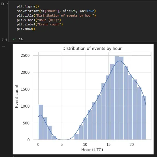
This confirms the presence of regular work-hour behavior and a smaller volume of off-hours activity.
Weekday Distribution
sns.countplot(x="dayofweek", data=df)
plt.title("Authentication events by day of week")
plt.xlabel("Day of week (0=Monday)")
plt.ylabel("Event count")
plt.show()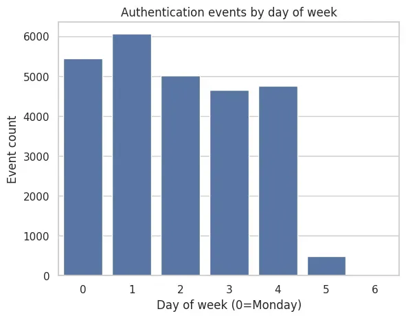
Most activity occurs on weekdays, with significantly lower volume during weekends.
Authentication Failures
sns.countplot(x="is_failure", data=df)
plt.title("Successful vs Failed Authentication Attempts")
plt.xlabel("Failure (1) / Success (0)")
plt.ylabel("Event count")
plt.show()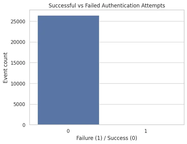
Failures are rare, which is expected in a healthy environment and reinforces their usefulness as anomaly signals.
IP Novelty per User
Finally, the distribution of user_ip_count highlights the presence of rare behavior:
sns.histplot(df["user_ip_count"], bins=30, kde=True)
plt.title("Distribution of user–IP frequency")
plt.xlabel("user_ip_count")
plt.ylabel("Event count")
plt.show()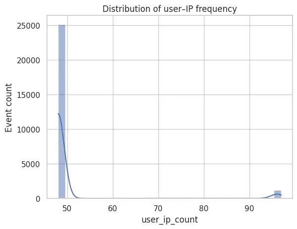
The distribution of user_ip_count is highly skewed: most authentication events originate from frequently observed user–IP pairs, while a small tail captures rare combinations. These low-frequency events provide a strong novelty signal for unsupervised anomaly detection.
Summary of Observations
Across these views, the dataset exhibits:
- Strong temporal regularity.
- Stable per-user baselines.
- Rare but meaningful deviations.
These properties are precisely what unsupervised anomaly detection models rely on to distinguish normal behavior from outliers.
Why This Step Matters
Anomaly detection is not about finding “bad events”. It is about learning what normal behavior looks like.
By:
- Keeping Elasticsearch as the system of record.
- Extracting only authentication-related events.
- Deriving interpretable behavioral features.
We create a robust foundation for detecting unknown and subtle deviations.
What’s Next
With behavioral features in place, the next step is to train a model to learn normal authentication behavior.
In Part 2, I will:
- normalize the feature space
- train an autoencoder using PyTorch
- analyze reconstruction error and anomaly scores
This completes the transition from logs to learned behavior.
Part 2: Unsupervised Anomaly Detection on Authentication Telemetry
Full code available: engineering-security-ml